오늘은 Autoencoder로 MNIST 데이터 생성해보는 과정을 말씀드리고자 합니다.
우선적으로 아래 예제 코드를 가지고 실행한 결과는 다음과 같습니다.
예제 코드)
# 차원축소 예제: 3차원 롤 데이터를 생성해서 autoencoder를 이용해서 2차원으로 표현하는 코드
import numpy as np
import matplotlib . pyplot as plt
def make_a_roll ( num_data ): # 롤 데이터 생성
f = 3
unit_length = np . linspace ( 0 , 1 , num_data )
t = f * unit_length * 3.14
x = np . sin ( t ) * ( unit_length + 0.5 ) + np . random . randn ( num_data ) * 0.01
z = np . cos ( t ) * unit_length + np . random . randn ( num_data ) * 0.01
y = + np . random . randn ( num_data ) * 0.3
r = unit_length
g = - ( 2 * ( unit_length - 0.5 )) ** 2 + 1
b = 1 - unit_length
X = np . array ([ x , y , z ])
C = np . array ([ r , g , b ])
return X . T , C . T
m = 150 #생성 데이터 개수
X , color = make_a_roll ( m )
fig = plt . figure ()
ax = fig . add_subplot ( 111 , projection = '3d' )
ax .scatter( X [:, 0 ], X [:, 1 ], X [:, 2 ], c = color , marker = 'o' , s = 15 )
plt . show ()
from tensorflow.keras import models
from tensorflow.keras import layers
enc = models.Sequential([layers.Dense( 2 , input_shape = [ 3 ],
activation = 'elu' )])
dec = models.Sequential([layers.Dense( 3 , input_shape = [ 2 ],
activation = 'elu' )])
AE = models.Sequential([ enc , dec ])
AE .compile( loss = 'mse' )
AE .summary() #Autoencoder model (encoder=4*2, decoder=3*3)
history = AE .fit( X , X , epochs = 10 ) #training (epoch=30)
plt . plot ( history .history[ 'loss' ], 'b-' ) #training error
plt . show ()
reduced = enc .predict( X ) # 생성된 2차원 데이터
plt . scatter ( reduced [:, 0 ], reduced [:, 1 ], color = color )
plt . show ()
결과)
결과 분석
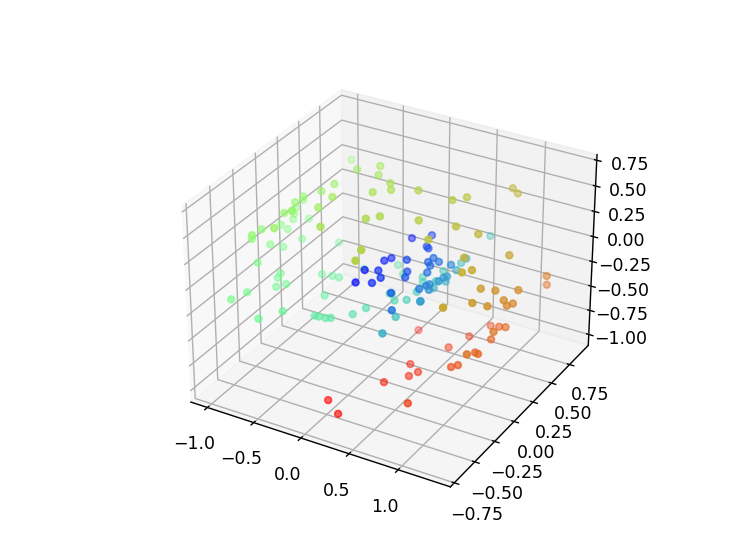
3차원 데이터 시각화
처음 생성된 3차원 롤 데이터는 나선형 형태를 띠며, 각 데이터 포인트는 다양한 색상을 가집니다.
이 시각화를 통해 데이터가 균일하게 분포되어 있음을 확인할 수 있습니다.
Autoencoder 모델 학습
모델 학습 과정에서 손실 값이 점차 감소하는 것을 확인할 수 있습니다. 이는 모델이 데이터의 중요한 특성을 학습하고 있음을 나타냅니다.
10 에포크 동안의 학습 후 손실 값이 안정화되며, 이는 모델이 적절히 수렴했음을 의미합니다.
차원축소 결과
인코더를 통해 축소된 2차원 데이터는 원래의 3차원 데이터와 유사한 구조를 유지합니다.
시각화 결과, 2차원 데이터 역시 나선형 형태를 띠며, 각 데이터 포인트의 색상 분포가 원래의 3차원 데이터와 일치합니다.
이는 Autoencoder가 데이터의 중요한 특성을 잘 학습하여 차원축소를 효과적으로 수행했음을 보여줍니다.
이제는 이러한 결과를 가지고 MNIST 데이터 생성해보겠습니다.
import numpy as np
import tensorflow as tf
from tensorflow.keras.datasets import mnist
from tensorflow.keras import layers, models
import matplotlib . pyplot as plt
# MNIST 데이터 로드 및 전처리
( x_train , _ ), ( x_test , _ ) = mnist.load_data()
x_train = x_train .astype( 'float32' ) / 255.0
x_test = x_test .astype( 'float32' ) / 255.0
x_train = x_train .reshape(( len ( x_train ), np . prod ( x_train .shape[ 1 :])))
x_test = x_test .reshape(( len ( x_test ), np . prod ( x_test .shape[ 1 :])))
# Autoencoder 모델 구성
encoding_dim = 32
input_img = layers.Input( shape = ( 784 ,))
encoded = layers.Dense( encoding_dim , activation = 'relu' )( input_img )
decoded = layers.Dense( 784 , activation = 'sigmoid' )( encoded )
autoencoder = models.Model( input_img , decoded )
autoencoder .compile( optimizer = 'adam' , loss = 'binary_crossentropy' )
# 인코더 모델
encoder = models.Model( input_img , encoded )
# 디코더 모델
encoded_input = layers.Input( shape = ( encoding_dim ,))
decoder_layer = autoencoder .layers[ - 1 ]
decoder = models.Model( encoded_input , decoder_layer ( encoded_input ))
# 모델 학습
autoencoder .fit( x_train , x_train , epochs = 50 , batch_size = 256 , shuffle = True , validation_data = ( x_test , x_test ))
# 차원축소된 데이터 얻기
encoded_imgs = encoder .predict( x_test )
decoded_imgs = decoder .predict( encoded_imgs )
# 결과 시각화
n = 10
plt . figure ( figsize = ( 20 , 4 ))
for i in range ( n ):
# 원본 이미지
ax = plt . subplot ( 2 , n , i + 1 )
plt . imshow ( x_test [ i ].reshape( 28 , 28 ))
plt . gray ()
ax . get_xaxis (). set_visible ( False )
ax . get_yaxis (). set_visible ( False )
# 재구성된 이미지
ax = plt . subplot ( 2 , n , i + 1 + n )
plt . imshow ( decoded_imgs [ i ].reshape( 28 , 28 ))
plt . gray ()
ax . get_xaxis (). set_visible ( False )
ax . get_yaxis (). set_visible ( False )
plt . show ()
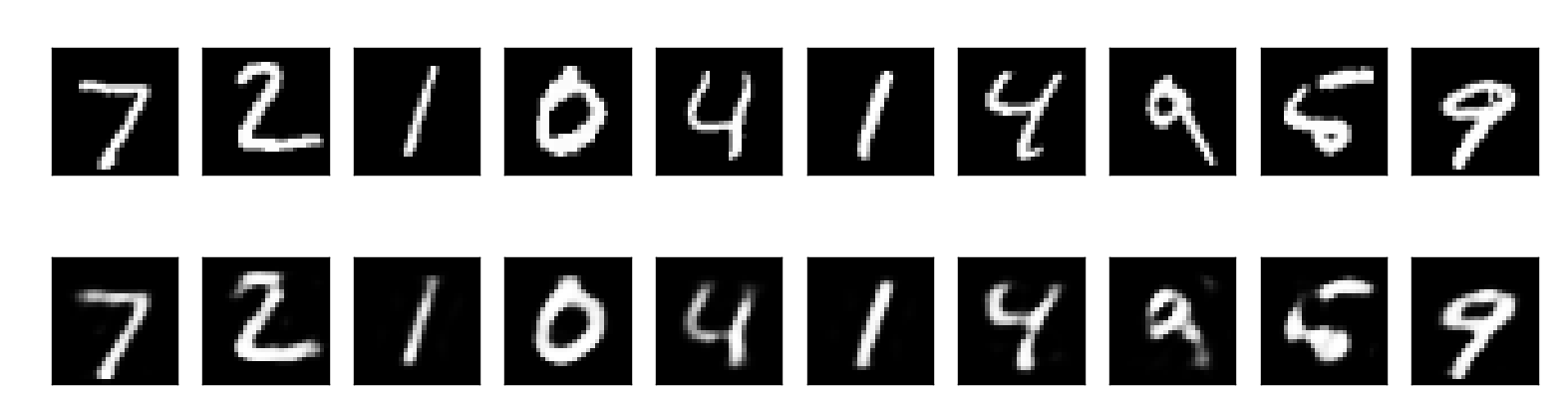
결과
코드에 대한 결과 정리는 다음과 같습니다.
1) MNIST 데이터 차원축소
2) Autoencoder 모델 구성 및 학습
3) 결과 시각화
이상으로 글 마치겠습니다.
감사합니다.